Cauchy distribution
Description
The Cauchy distribution, named after Augustin Cauchy, is a continuous probability distribution. It is also known, especially among physicists, as the Lorentz distribution (after Hendrik Lorentz), Cauchy–Lorentz distribution, Lorentz(ian) function, or Breit–Wigner distribution. The Cauchy distribution
The Cauchy distribution is often used in statistics as the canonical example of a "pathological" distribution since both its expected value and its variance are undefined (but see § Explanation of undefined moments below). The Cauchy distribution does not have finite moments of order greater than or equal to one; only fractional absolute moments exist. The Cauchy distribution has no moment generating function.
In mathematics, it is closely related to the Poisson kernel, which is the fundamental solution for the Laplace equation in the upper half-plane.
It is one of the few distributions that is stable and has a probability density function that can be expressed analytically, the others being the normal distribution and the Lévy distribution.
Probability Density Function
The general formula for the probability density function of the Cauchy distribution is
where t is the location parameter and s is the scale parameter. The case where t = 0 and s = 1 is called the standard Cauchy distribution. The equation for the standard Cauchy distribution reduces to
Since the general form of probability functions can be expressed in terms of the standard distribution, all subsequent formulas in this section are given for the standard form of the function.
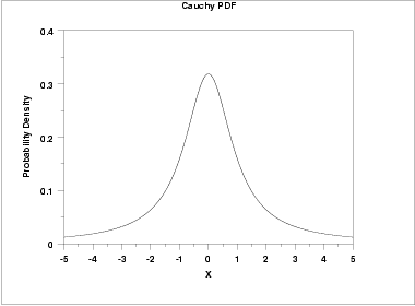
The following is the plot of the standard Cauchy probability density function.

Cumulative Distribution Function
The formula for the cumulative distribution function for the Cauchy distribution is
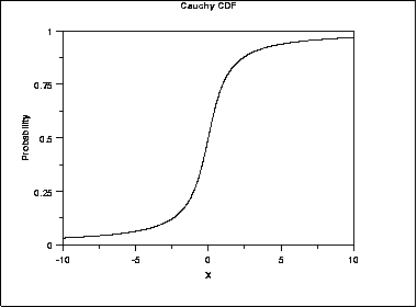
The following is the plot of the Cauchy cumulative distribution function.

...
Common Statistics
| Mean | The mean is undefined |
| Median | The location parameter t |
| Mode | The location parameter t |
| Range | −∞ to ∞ |
| Standard Deviation | The standard deviation is undefined |
| Coefficient of Variation | The coefficient of variation is undefined |
| Skewness | The skewness is 0 |
| Kurtosis | The kurtosis is undefined |
Parameter Estimation
The likelihood functions for the Cauchy maximum likelihood estimates are given in chapter 16 of Johnson, Kotz, and Balakrishnan. These equations typically must be solved numerically on a computer.
Comments
The Cauchy distribution is important as an example of a pathological case. Cauchy distributions look similar to a normal distribution. However, they have much heavier tails. When studying hypothesis tests that assume normality, seeing how the tests perform on data from a Cauchy distribution is a good indicator of how sensitive the tests are to heavy-tail departures from normality. Likewise, it is a good check for robust techniques that are designed to work well under a wide variety of distributional assumptions.
The mean and standard deviation of the Cauchy distribution are undefined. The practical meaning of this is that collecting 1,000 data points gives no more accurate an estimate of the mean and standard deviation than does a single point.