Houdini Micro Solvers

· Houdini MOC ·

TOC

• Preparation
• MicroSolvers
  • Gas Advect & Gas Advect Field
  • Gas Linear Combination
  • Gas Disturb Field
  • Gas Turbulence
  • Gas Dissipate
  • Gas Damp
  • Gas Blur
  • Gas Buoyancy
  • Gas Vortex Boost
  • Gas Particle to Field
  • Gas Field to Particle
  • Color Diffusion
  • Gas Analysis
• References

Micro Solvers are building blocks in Houdini simulation. Mostly they are doing one task in a clean way. SideFx’ fluid solvers from scratch tutorial and Pater Claes’ master theses about custom fields helps a lot for learning however there are tons of them and started to a bit confusing. Hence I make little list of these nodes with some examples attasched. It is first part and I am planning to prepare 3 parts in total.

Preparation

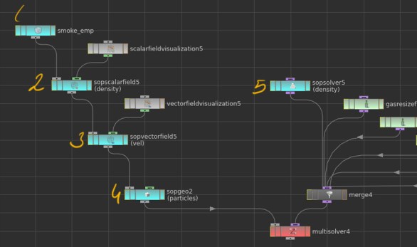
Lets start with multi solver as we will apply many micro solvers fin each time step. It has two inputs, objects (left) solvers (right). Objects to be processed will be as fallows:

1. Empty Objectis a container which can have various types of data attached to it.

2. The Scalar Field DOP creates a Scalar Field data that can be attached to simulation objects and manipulated by solvers. Scalar data can be density, temperature or any floating point number. Scalar field Visualization is attached to this node for field visualization.

3. The Vector Field DOP creates a Vector Field data that can be attached to simulation objects and manipulated by solvers. Same as previous one except in this node each voxel is giving a 3d vector instead float. For visualizing field vector field Visualization node is used.

4. Sop Geometry for importing external objects in to simulation. In our case it will be particles.

5. Sop Solver to feed simulation with density in each frame. Inside this solver, density source is imported and merged with, dop geometry.

Micro Solvers

Gas Advect & Gas Advect Field

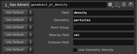
Evolves fields and geometry according to a specified velocity field. The fields and geometry will be moved by the velocity field for a distance proportional to the current solver timestep. In example below velocity drives density and particles. Velocity field needs to advect itself also, otherwise velocity grid will be static (will not change through simulation).

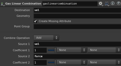
Gas Linear Combination

Combines multiple fields or geometry attributes together. In example masked force field (another SOP Vector Field) and velocity field added to velocity itself.

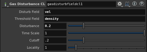
Gas Disturb Field

Introduces small amounts of change in momentum which cancels itself out over time, preserving the simulation’s general motion. In example velocity is disturbed according to density field

Gas Turbulence

Creates and applies a global turbulence field to the specified velocity field. This turbulent velocity field is modulated by the Control Field and lookup ramps provided.

Gas Dissipate

Deforms dissipation on the specified field. This will drive the fields value to zero. An optional control field can be used to affect when the dissipation occurs. In mid Example gas dissipation is enabled by evaporation, each timestep subtraction applied to density field. In right example min clamp applied

Gas Damp

The Gas Damp DOP scales the velocity field by a number between 0 and 1, thereby slowing down the motion in the simulation.

Gas Blur

The Gas Blur DOP blurs fields using an optionally time dependent blur kernel. In Example density field is blurred by gaussian with radius of 0,2.

Gas Buoyancy

Calculates an approximate buoyancy force dependent on the temperature field and updates a velocity field according to that force. In example gas buoyancy is driven by temperature. While left one’s temperature is static, right one’s temperature is advected by velocity hence buoyancy force is diffused through time.

Buoyancy force = ((l * (T-Ta)) * B
Ta = Given an ambient temperature
T= Temperature T
l = Buoyancy lift
B = buoyancy direction

Gas Vortex Boost

Applies confinement to a specific band of energy captured from the velocity field. Confinement force is applied for undoing the diffusion by amplifying existing vortices

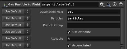
Gas Particle to Field

The Gas Particle to Field DOP copies a point attribute value from a particle system into a field. In example below, N attribute of points added to velocity field. Accumulated checkbox enables to replace or add to existing field.

Gas Field to Particle

Calculates the field value for each particle in the geometry. The resulting field values is then mixed with the particle’s attribute value to get the new attribute value. In example below particles stores density and velocity field of simulation. As post solution process, low dens particles are removed and color given based on velocity.

Color Diffusion

In following example, color is imported as vector field to simulation and diffused together.

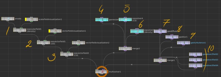
1. SOP Scalar Field for density import
2. SOP Vector Field for velocity import
3. SOP Vector Field for color import
4. Gas Resize
5. SOP Solver for merging source color field for first 15 frames
6. SOP Solver for merging source density field for first 15 frames
7. Gas Diffuse
8. Gas Blur
9. Gas Turbulence
10. Gas Advect nodes for velocity advect color density and itself

Gas Analysis

In following example Gas Analysis micro solver is used in order to calculate curl and curvature fields for more detailed fluid shape.

1. Importing points to sim.
2. Particles advected by velocity.
3. Normal curl and curvature fields are matched with reference vel field.
4. Gas Particle to Fieldparticle normals transfered to field with normal name.
5. Gas Analysis: curl analyses has been applied on normal field, output is curl
6. GasAnalysis2: curvature analyses has been applie to curl field, output is curvature
7. Gas Field Vop: inside vop, curl and curvature fields added to velocity field.

More information about Gas Analysis micro solver, little bit Houdini help and little bit Wikipedia;

Gas Analysis The Gas Analysis DOP computes various analytic properties of the input field to produce the output field.

• Curvature is the amount by which a geometric object such as a surface deviates from being a flat plane.
• Curl (rot) outputs a vector that lies in the axis of rotation of the field and has magnitude proportional to the field’s rotation speed at that point.The direction of the curl is the axis of rotation. If the vector field represents the flow velocity of a moving fluid , then the curl is the circulation density of the fluid.
• Gradient can be used to measure how a scalar field changes in other directions. The magnitude of the gradient will determine how fast specified field will move in that direction. For example, if temperature rises faster over a shorter distance, it will create a bigger gradient.
• Laplace’s equation in fluid dynamics describes the behavior of gravitational and fluid potentials.
• Divergence represents the volume density of the outward flux of a vector field from an infinitesimal volume around a given point. As an example, consider air as it is heated or cooled. The velocity of the air at each point defines a vector field. While air is heated in a region, it expands in all directions, and thus the velocity field points outward from that region. The divergence of the velocity field in that region would thus have a positive value. While the air is cooled and thus contracting, the divergence of the velocity has a negative value.
• Normalize destination is set to the source after normalizing the length of the source vector.
• Length the scalar field is set to the length of the vector field at each location. The length is calculated by measuring the slope of increasing values

The Gas Match Field DOP creates, resizes, and resamples as necessary to ensure the data matching the given name exists as a field of the same resolution and size as the reference field. In this example this node is used to match curl, normal and curvature fields with vel field.

References

• SideFx’ fluid solvers from scratch tutorial
• Pater Claes’ master theses about custom fields
• https://en.wikipedia.org/wiki/Gradient
• https://en.wikipedia.org/wiki/Curl_(mathematics)
• https://en.wikipedia.org/wiki/Curvature
• https://en.wikipedia.org/wiki/Laplace%27s_equation